1st NextGenTriggers Hackathon

Download and install

MadGraph is given as is, no proper installation is required.

Software prerequisites

Python 3.7+;
Fortran compiler (gfortran v4.6+);
other optional tools can then be installed through the MadGraph prompt.

Installation

Here you can find the official MadGraph repository. You have two possibilities:

clone the repository and checkout the latest version tag v3.6.2:

git clone --depth 1 --branch v3.6.2 https://github.com/mg5amcnlo/mg5amcnlo.git

download a tarball and unpack it locally:

wget https://github.com/mg5amcnlo/mg5amcnlo/archive/refs/tags/v3.6.2.tar.gz
mkdir -p mg5amcnlo
tar xzf v3.6.2.tar.gz -C mg5amcnlo

Now cd into it:

cd mg5amcnlo

and explore the structure with ls or tree (if you have it installed):

ls -1

will return:

aloha
Analyses
bin
HELAS
input
INSTALL
LICENSE
madgraph
MadSpin
mg5decay
models
PLUGIN
README.md
Template
tests
UpdateNotes.txt
vendor
VERSION

Let’s now study separately the folders:

bin: it contains the main executable to run MadGraph: mg5_aMC;
input: it contains the mg5_configuration.txt file, that specifies several general settings;
models: there are already several models pre-installed, including the Standard Model (sm) and the Standard Model ready for NLO calculations (loop_sm), have a look at the file listings of each of them, you will find many python files, that are automatically written by Feynrules when exporting the model in UFO format;
PLUGIN: this directory will contain any installed external plugins (we will have a look at it later in the hackaton).

Start MadGraph

./bin/mg5_aMC

There is no need to start it from the same directory, and it is not If you want a certain python version, then either use virtualenv, or specify python from the command line:

python ./bin/mg5_aMC

As you can see, MadGraph is a command-line tool, it has a prompt with tab-completion, waiting for your commands.

Exercise 1: let’s start the tutorial

Now type:

> tutorial

This will start the main tutorial and it will go through the main aspects of the code:

how to generate a process;
how to display the list of diagrams and processes;
how to specify multiple processes;
how to write a decay chain;
how to export the process code;
how to run/launch an event generation.

Focus: the `display_diagrams` command

This command allows to display the different Feynman diagrams making up the process. The resulting PDFs are saved in the system temporary folder (/tmp on Linux). Notice that this command may not work on Windows Subsystem for Linux, without an X-server enabled.

TODO
Explore this command for different processes. Try also display_processes.

Focus: the `output` command

This command will create a folder with a certain name, in which it will save all the generated code (remember: MadGraph is a meta-code). You can explore the folder by cding into it:

bin
Cards
Events
HTML
index.html
lib
madevent.tar.gz
MGMEVersion.txt
README
README.systematics
Source
SubProcesses
TemplateVersion.txt

where:

bin/generate_events does the same as the launch <this_folder> from the main prompt;
Cards contains the cards that can be modified also offline;
index.html and HTML contain the website dashboard showing informations on the various runs;
lib, Source, SubProcesses contain MadGraph internals;
madevent.tar.gz contains the generated code in this folder: it is exactly a copy of this folder.

Focus: particles and multiparticles

In MadGraph, each particle has a name, a is the photon, g the gluon, c the charm quark, e+ the positron, h the higgs boson, ecc. One can consider the related antiparticle by appending a ~ to the particle name, so that t~ is the anti-top quark. Additionally, when starting MadGraph a set of multiparticles is displayed: they are aliases referring to a set of different particles. E.g. the proton is not an elementary particle, but one could define the multiparticle p to contain the set g u c d s u~ c~ d~ s~, meaning the lightest quarks and the gluon. When generating processes, multiparticles are used so that the process generator will try any member of the multiparticle set when trying the processes, and if multiple multiparticles are specified in a single process generation, all the different combination in between their sets are tried.

Exercise 2: Cards meaning

How do you change?

top mass
top width
W mass
beam energy
pt cut on the lepton

TODO
Try to change them!

TIP
Cards parameter can be set via the set command during the question time, and tab-completion is enabled:
set MT 170
set ebeam 500

Param card

The param card contains the various parameters that are settable according to the model: masses, couplings, and widths.

TODO
Have a look at the Cards/param_card.dat

Run card

The run card contains the parameters strictly related to the run: beams energies, cuts, and so on (even the run tag).

TODO
Have a look at the Cards/run_card.dat

Exercise 3: Syntax

What is the meaning of the order QED/QCD?
Learn the difference between:
- p p > t t~
- p p > t t~ QED=2
- p p > t t~ QED=0
- p p > t t~ QCD^2==2

TODO
Generate p p > t t~, and do display_diagrams, is anything missing?

By default, MadGraph takes the lowest order in QED, so p p > t t~ is equivalent to p p > t t~ QED=0. While with p p > t t~ QED=2 we have additional diagrams with photon/Z exchange.

TODO
Generate the process p p > t t~ with different QED orders and compute the cross-section. Is the QED contribution high?

Syntax QED<=2 is the same as QED==2. While QCD^2==2 return the interference between the QCD and QED diagram.

TODO Try to compute it!

TODO
Try to generate the following processes and observe the number of created diagrams in each case:

p p > w+ w- j j

p p > w+ w- j j QED=2

p p > w+ w- j j QED=4

p p > w+ w- j j QCD=0

p p > w+ w- j j QCD=2

p p > w+ w- j j QCD=4

What is `WEIGHTED`

It is a label to indicate the maximum order of diagrams to generate, considering that:

QCD: WEIGHTED is 1;
QED: WEIGHTED is 2.

TODO
Try to generate p p > t t~ WEIGHTED=4, and observe the diagrams.

Exercise 4: Syntax

Generate the cross-section and the distribution (invariant mass) for:

p p > e+ e-
p p > z, z > e+ e-
p p > e+ e- / z
p p > e+ e- $ z

TIP
To have automatic distributions, install MadAnalysis:
mg5> install MadAnalysis5
Then, generated plots are shown in the MadAnalysis card (and the prompt will now ask if you want to modify it), do the runs with sufficient number of events, like 100k, and generate the plot M from 0 to 200, with 100 bins:
plot M(e-[1] e+[1]) 100 0  200 [logY ]
Output plots can be found in $PROC_DIR/HTML/run_<n>/tag_1_MA5_PARTON_ANALYSIS_analysis1/Output/PDF/MadAnalysis5job_0. You may need Root:
dnf install root

Syntax examples can be found at the following pages:

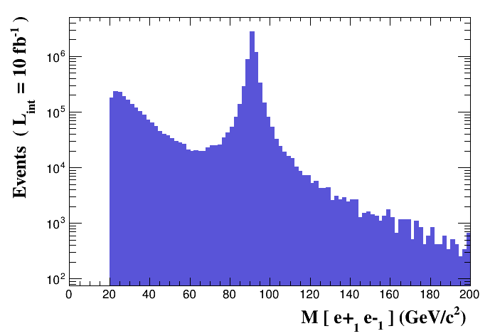
`p p > e+ e-`

We see the Z peak. Invariant mass pp_epem

`p p > z, z > e+ e-`

We see the Z peak. Invariant mass pp_z_epem

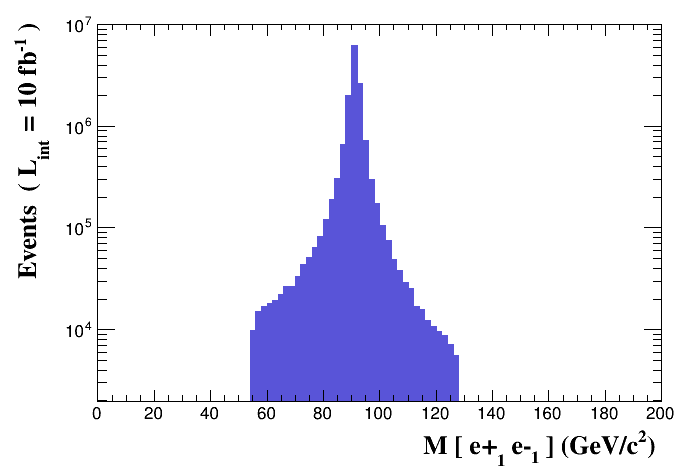
The breadth of the distribution depends on the value of the Z width, and on the parameter bwcutoff of the run card (set to 15 by default), which is a cut on how far a particle can be off-shell. $|M^\ast - M| < BW_\text{cut} \cdot \Gamma$

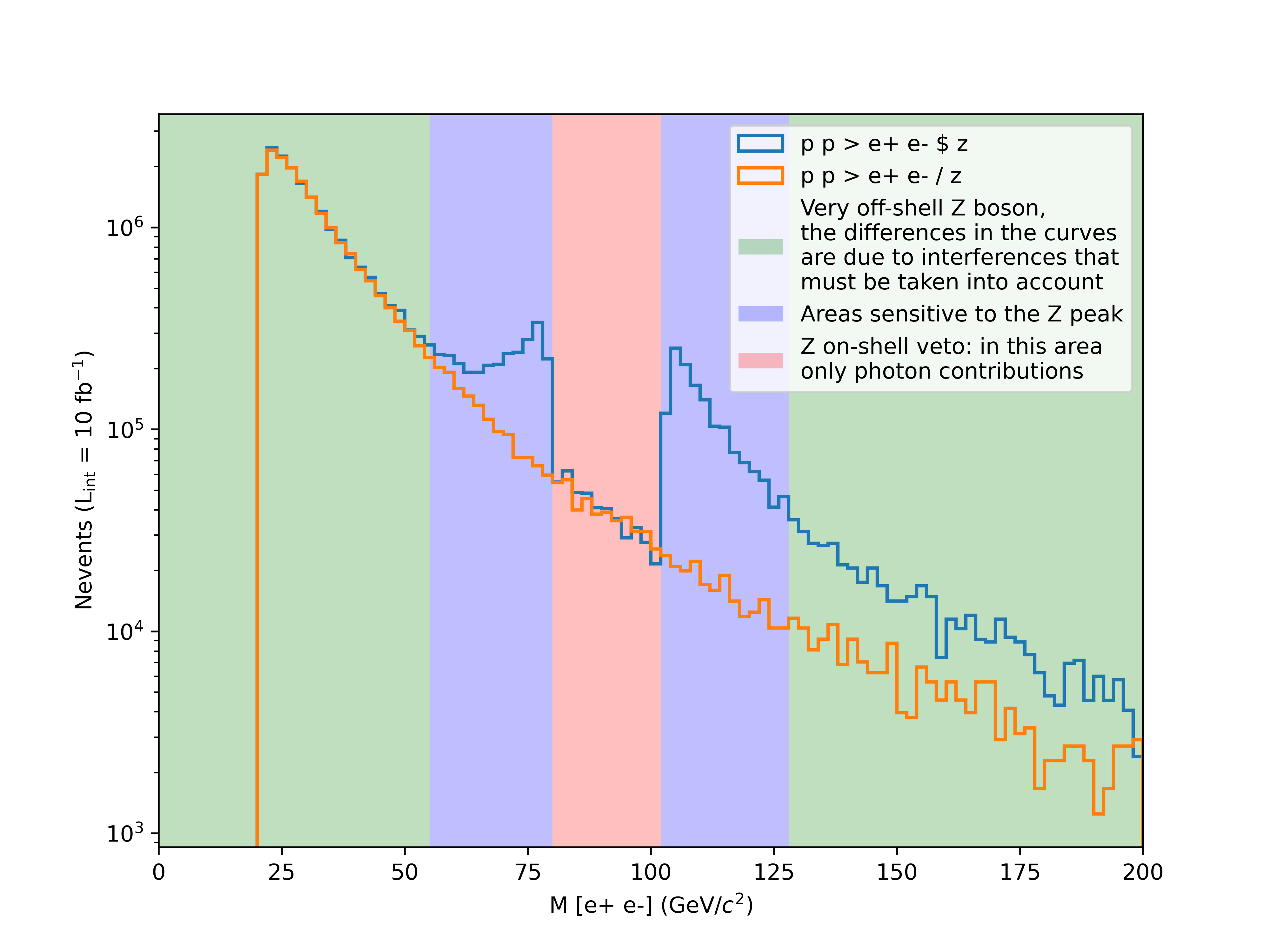
`p p > e+ e- / z`

We don’t see the Z peak, and we don’t have photon/Z diagrams interference Invariant mass pp_epem-z

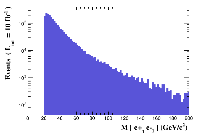
Forbids any Z.

CAUTION
Avoid this syntax, since it leads to a violation of gauge invariance.

`p p > e+ e- $ z`

We don’t see the Z peak, but we have photon/Z diagrams interference. Invariant mass pp_epem-no_s_z

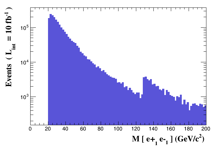
The $ forbids the Z to be on-shell, but the photon invariant mass can be at $m_Z$. This is basically a Z-on-shell veto, and only the photon is contributing in the $m_Z$ region.

Note on the distribuition

Notice that the correct distribution is the one for p p > e+ e-, while we can also see that more or less the sum of:

p p > z, z > e+ e-
p p > e+ e- $ z

resembles it.

[!CAUTION] Syntaxes like:

p p > z > e+ e- (ask one s-channel Z);

p p > e+ e- / Z (forbids any Z);

p p > e+ e- $$ z (forbids any Z in s-channel);

are not gauge invariant, and can provide unphysical distributions. Prefer the other syntaxes.

Indeed, let’s have a look at the differences in the mass invariant distribution between the syntaxes p p > e+ e- / z and p p > e+ e- $ z: the first one will exclude the presence of the Z boson, so no interference is computed, while the second would just exclude on-shell Z boson in the range determined by the value of bwcutoff. Just to exaggerate the result, we will set bwcutoff to 5 (way to small for practical purposes), but it will show how different the tails would look like.

Exercise 5: Automation

Using the prompt is boring. MadGraph provides a way to use scripts to automate the runs. Basically, you write every command as a separate line in a text file, and MadGraph would execute them one after the other. Whenever there are questions in the prompt, if the answer is not present, the default is taken automatically. Comments are prepended with # (Python way). Submit the script via:

./bin/mg5_aMC myscript.txt

TIP
I like to keep generate and launch scripts separated, but one can write a single script performing both the process generation and the running.

Example of a generate script

import model sm # notice that the sm is imported by default
generate p p > t t~
output mytestdir

Example of a launch script

launch mytestdir # specify the name of the folder in the current cwd
set ebeam1 4000
set ebeam2 4000
set MT 170
launch # perform a second run
set MT 172
launch
set MT 174
launch
set MT 176
launch
set MT 178
launch
set MT 180

You can also specify the name of the run for each launch, so that you can track it down:

launch mytestdir -n run_MT170
set ebeam1 4000
set ebeam2 4000
set MT 170
launch -n run_MT172
set MT 172
launch -n run_MT174
set MT 174
launch -n run_MT176
set MT 176
launch -n run_MT178
set MT 178
launch -n run_MT180
set MT 180

TODO
Open the index.html and track down the run results.

Scan syntax

One can also use the scan syntax to perform automatic scans over multiple parameters in a single launch. The scan syntax support python lists of floats, or even python list comprehension:

set MT scan:[170,172,174,176,178];
set MT scan:[170 + 2*i for i in range(5)].

Nested scan over multiple parameters

The following syntax:

set MT scan:[170,172]
set MH scan:[123,125,127]

Will scan over all possible pairs of MT and MH values.

Parallel scan over multiple parameters

The following syntax:

set MT scan1:[170,172]
set MH scan1:[123,125]

Will scan over the parallel pairs of MT and MH values.

Exercise 6: Decay

Observe the following decay syntax:

generate p p > t t~ h, (t > w+ b, w+ > e+ ve), (t~ > w- b~, w- > e- ve~)

This will generate the first process, and then prepare the decay of the final states t, t~.

TODO
Run the following:
generate p p > t t~, t > w+ b, t~ > w- b~
output
launch
set mt scan:range(170,181,2)
And inspect the cross section. Why is it increasing?

This happens because the top width is kept fixed, however, its mass changes, so it needs to be updated: use set wt auto to take care of that automatically (only leading order contributions).

Exercise 7: Gridpacks

When running ./bin/generate_events, MadGraph automatically recompiles the code inside the folder for the set of parameters and settings that have been chosen in the cards. However, this implies that this is done every run and it can be quite time-consuming, especially if we consider that most of MadGraph jobs are splitted across a grid of machines. Additionally, the interactive approach, despite the usage of automation script, is a non-trivial overhead for large-scale production. For this reason, MadGraph has the possibility to create a packaged version of the generated code that contains all the binaries already compiled, includes all the settings and parameters set, and that is ready to be shipped on grid workers, hence the name: gridpack.

To generate a gridpack, set the option from the run card when running ./bin/generate_events:

set gridpack True

At the end of the run, that will not produce any events, you will have a new archive inside the main process folder named as run_XX_gridpack.tar.gz. You can move the archive in another location and unpack it. It will produce:

the folder madevent containing the compiled code and all the files useful to run the event generation;
the file run.sh, an executable script that requires two arguments: the number of events to generate and the random number generator seed.

TODO
Run run.sh and see what happens.

Running run.sh will produce the events.lhe.gz file in the current working directory.

Exercise 8: Where are the results?

Where are the output files?

Each run done with ./bin/generate_events will create a folder inside Events named after the run number (or the name passed by the -m option of the launch command). That folder contains a file banner which will report the cross section result along with a dump of both the Param and Run cards.

LHE file

Both runs with ./bin/generate_events and with gridpacks will produce a file containing the generated events in the Les Houches Event file (LHE) format, which is the current standard to store process and event information from parton-level event generators. The file contains an header with the generator and model information (basically a dump of the Param and Run cards) followed by the events record, containing multiple blocks. Each event is a list of particles and each particle is represented by the sequence of the following attributes: ID, status, mother1, mother2, color, anticolor, px, py, pz, E, mass, lifetime, and spin, e.g.:

-11  1    3    3    0    0 -2.3393803385e+01 -7.4187481776e+00 -1.5274153214e+02 1.5470062541e+02 0.0000000000e+00 0.0000e+00 1.0000e+00

This line tells you that a positron (-11) is an outgoing particle (1) with Z as its mother (mother1 and mother2 are pointing to the 3rd - 3 - particle of the same record, which is a Z boson - ID is 23), with no color (color and anticolor are both 0), and the following four-momentum, mass, lifetime (it is stable) and spin.

Getting familiar with MadGraph